Tính GDP thực

June 10, 2017June 10, 2017 ~ kinhteking ~ Leave a comment

Có hai cách phổ biến để tính GDP thực:
1) Dựa trên giá của năm cơ sở
2) Liên kết chuỗi dựa trên tăng trưởng của sản lượng thực

Phần lớn các quốc gia hiện dùng phương pháp thứ hai vì hạn chế của phương pháp thứ nhất chính là việc không tính đến sự thay đổi trong tỷ trọng giữa các nhóm hàng hóa. Ví dụ như, máy tính càng ngày càng rẻ trong khi sản lượng máy tính tăng rất nhiều. Nếu dùng giá của những năm trước, tỷ trọng của tiêu dùng máy tính trong GDP thực rất cao.

Để hiểu rõ hơn về về hai cách tính sản lượng thực, xem giải thích của GS Menzie David Chinn: https://www.dropbox.com/s/4ukwhnts2c1p14q/chain_GDP.pdf?dl=0

Cơ bản: Mô hình Tổng cầu và Tổng cung AD-AS

June 22, 2016June 16, 2017 ~ kinhteking ~ 2 Comments

Gần đây, nhà kinh tế Olivier Blanchard có để xuất bỏ mô hình AD-AS khỏi giáo trình giảng dạy kinh tế vĩ mô trung cấp ở bậc đại học (Blanchard nguyên là kinh tế trưởng của IMF) (Xem ở đây). Lý do chính là bởi mô hình AD-AS dễ gây nhầm lẫn và khiến cho sinh viên cảm thấy khó hiểu.

Một mục tiêu quan trọng của mô hình AD-AS là để minh họa làm thế nào nền kinh tế TỰ trở lại mức tiềm năng mà không cần sự can thiệp của chính sách, thông qua một cơ chế mà, theo Blanchard, ít liên quan đến thực tế: ví dụ, sản lượng giảm ==> mức giá giảm ==> mức cung tiền thực tăng vì không có thay đổi ở mức cung tiền danh nghĩa ==> lãi suất giảm ==> tăng cầu ==>tăng sản lượng. Blanchard cho rằng quy trình này gồm một chuỗi những sự kiện phức tạp mà tính thực tế của nó rất đáng ngờ. Trung tâm của sự điều chỉnh này chính là giả định cung tiền danh nghĩa không đổi. Giả định này ít thực tế vì các NHTW hiện đại điều hành dựa trên công cụ lãi suất chứ không phải mức cung tiền. Ngoài ra, cơ chế tự điều chỉnh này dường như không hoạt động trong suốt 7 năm vừa qua.

Bài viết này sẽ xem lại mô hình AD-AS để hiểu lý do tại sao Olivier đề xuất như vậy, dựa trên giáo trình kinh tế vĩ mô của Blanchard và Johnson (ISBN 13: 978-0-273-76633-9).

ĐƯỜNG TỔNG CUNG AS

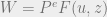
Đường tổng cung AS minh họa tác động của sản lượng vào mức giá. Chúng ta bắt đầu xây dựng đường tổng cung từ phương trình quyết định mức giá như sau:

$P=(1+m)W$ (1)

Mức giá P được quyết định bởi các hãng theo tỷ lệ của mức lương danh nghĩa. Tỷ lệ này là (1+m) với m là mức tăng giá so với chi phí (mark-up). Nếu m=1 hay 100%, nghĩa là nếu mức lương trung bình là 50 nghìn đồng trên 1 sản phẩm, thì mức giá là 100 nghìn đồng.

Mức lương danh nghĩa phụ thuộc vào lạm phát kỳ vọng $P_{e}$ , tỷ lệ thất nghiệp $u$ , và các nhân tố khác ảnh hưởng đến lương $z$ (như trợ cấp thất nghiệp, hay là liên đoàn)

$W = P^{e} F(u,z)$ (2)

Kết hợp hai phương trình (1) và (2), phương trình đường tổng cung có dạng:

$P=P^{e}(1+m)F(u,z)$ (3)

Vai trò của tổng sản lượng hiện diện gián tiếp trong phương trình trên thông qua ảnh hưởng đến tỷ lệ thất nghiệp (Có thể tham khảo định luật Okun).

Một đơn giản hóa mang tính minh họa là giả định để sản xuất một sản phẩm cần MỘT lao động, ta có thể thấy mối liên hệ giữa tỷ lệ thất nghiệp và tổng sản lượng như sau:

$u=\frac{L-N}{L}=1-\frac{N}{L}=1-\frac{Y}{L}$

với L là lực lượng lao động và N là số lao động có việc làm.

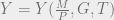
Do đó, ta có thể viết lại phương trình (3) như sau:

$P=P^{e}(1+m)F(1-\frac{Y}{L},z)$ (4)

Hình 1 minh họa đường tổng cung AS. Chú ý rằng khi sản lượng ở mức tiềm năng, $Y=Y^{n}$ , mức giá sẽ bằng với mức gía được kỳ vọng $P=P^{e}$ . Tại sao? Tỷ lệ thất nghiệp tự nhiên, đồng nghĩa với sản lượng ở mức tiềm năng, được định nghĩa là tỷ lệ thất nghiệp tồn tại khi mà mức giá bằng với mức giá kỳ vọng.

Hình 1: Phương trình đường tổng cung

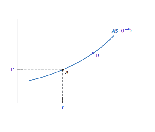
Hai tính chất quan trọng của đường tổng cung:

Tại một mức giá kỳ vọng cho trước, nếu sản lượng tăng, mức giá sẽ tăng (Hình 1: Dịch chuyển từ điểm A đến điểm B)

Sản lượng tăng ==>việc làm tăng ==> Thất nghiệp giảm ==> Mức lương danh nghĩa tăng ==> giá tăng (Phương trình 2 và 3)

Tại một mức thất nghiệp cho trước, nếu mức giá kỳ vọng tăng, giá sẽ tăng theo một tỷ lệ tương ứng (1:1)

Nếu mọi người kỳ vọng giá tăng ==> yêu cầu mức lương danh nghĩa cao hơn khi ký hợp đồng lao động mới hoặc khi có cơ hội đàm phán lại mức lương ==> chi phí tăng ==> doanh nghiệp tăng giá ==> mức giá tăng trong nên kinh tế (Hình 2: Điểm A đến điểm A’)

Hình 2: Mức giá kỳ vọng tăng

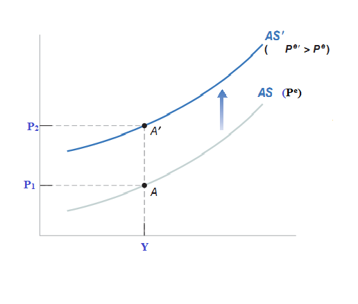
Do vậy cần lưu ý rằng: Mỗi đường tổng cung tương ứng với một mức giá kỳ vọng. Những thay đổi trong mức giá kỳ vọng sẽ làm đường tổng cung dịch chuyển. Mức giá kỳ vọng tăng làm AS dịch chuyển lên trên, trong khi đó sự giảm của kỳ vọng làm AS dịch chuyển xuống dưới.

ĐƯỜNG TỔNG CẦU AD

Đường tổng cầu AD thể hiện tác động của giá vào tổng sản lượng. Phương trình đường tổng cầu có dạng sau:

$Y=Y(\frac{M}{P}, G,T)$

Nhắc lại, để xây dựng đường tổng cầu, chúng ta sử dụng mô hình IS-LM (cân bằng thị trường hàng hóa và thị trường tiền tệ).

Phương trình IS: (sủ dụng mô hình nền kinh tế đóng để minh họa)

$Y=C+I(i)+G$

với $i$ là mức lãi suất. Tổng sản lượng bằng tổng cầu hàng hóa.

Phương trình LM:

$\frac{M}{P}=f(Y,i)$

Vế trái là cung tiền, còn vế phải là cầu tiền phụ thuộc vào thu nhập và lãi suất.

Khi mức giá $P$ tăng lên, cung tiền thực $\frac{M}{P}$ giảm vì lượng cung tiền danh nghĩa $M$ không đổi. Hệ quả là đường LM sẽ dịch chuyển sang trái, làm lãi suất tăng lên và tổng cầu giảm.

Hình 3: Mô hình IS-LM

AD1

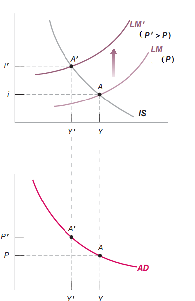
Hai đặc tính của đường tổng cầu

1.Khi giá tăng, tổng cầu giảm ==> đường AD có hướng dốc xuống (Hình 3).

2.Các yếu tố ngoài giá mà làm dịch chuyển đường IS (ví dụ như chính sách tài khóa) và đường LM (ví dụ như chính sách tiền tệ) cũng sẽ làm dịch chuyển đường AD

Tăng cung tiền ==> LM dịch sang phải ==> AD cũng dịch sang phải
Tăng chi tiêu chính phủ ==> IS dịch sang phải ==> AD cũng dịch sang phải
Tăng thuế ==> IS dịch sang trái ==> AD cũng dịch sang trái.
Giá thay đổi ==> LM dịch chuyển ==> thay đổi lên xuống trên đường AD (Ví dụ điểm A đến điểm A’), chứ AD không di chuyển.

KẾT HỢP TỔNG CUNG- TỔNG CẦU AS-AD

Cơ chế tự điều chỉnh của AD-AS

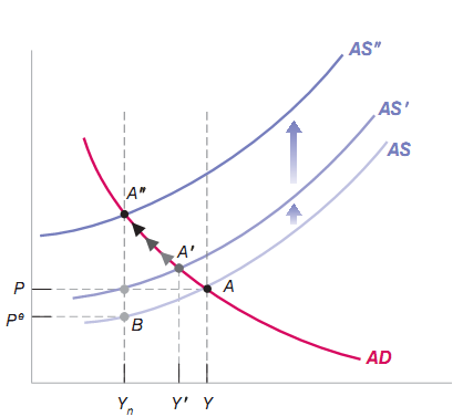
Hình 4 kết hợp hai đường tổng cầu và tổng cung để minh họa cơ chế tự điều chỉnh.

Trong ngắn hạn không phải khi nào nền kinh tế cũng ở mức sản lượng tiền năng. Giả sử nền kinh tế hiện ở điểm A với $Y> Y_{n}$ sản lượng lớn hơn sản lượng tiềm năng. Tại điểm này mức giá cao hơn mức giá kỳ vọng (Vì $P=P^{e}$ khi $Y=Y^{e}$ ). Do vậy, khi người lao động (hoặc những người quyết định lương) được xét lại mức lương mới hoặc ký mới hợp đồng lao động, họ thường sẽ thiết lập mức kỳ vọng mới về giá cao hơn so với trước ( $P_{e'}>P_{e}$ ). Như được đề cập ở trên, mỗi đường tổng cung tương ứng với 1 mức giá kỳ vọng. Khi mức giá kỳ vọng tăng, đường tổng cung dịch chuyển sang trái, đẩy mức giá lên cao hơn. Quý trình này tiếp tục và đưa nền kinh tế đến đểm $A''$ và sản lượng trở về mức tiềm năng $Y_{n}$ , do đó tỷ lệ thất nghiệp trở lại bằng với tỷ lệ thất nghiệp tự nhiên (Xem hình 3 về sự dịch chuyển của LM do giá thay đổi). Lập luận tương tự nếu $Y< Y_{n}$ )

Hình 4: Cơ chế tự điều chỉnh

ADAS

Blanchard cho rằng quy trình này gồm một chuỗi những sự kiện phức tạp mà tính thực tế của nó rất đáng ngờ. Trung tâm của sự điều chỉnh này chính là giả định cung tiền danh nghĩa không đổi. Giả định này ít thực tế vì các NHTW hiện đại điều hành dựa trên công cụ lãi suất chứ không phải mức cung tiên. Ngoài ra, quan điểm “tự điều chỉnh” dường như không hoạt động trong suốt 7 năm vừa qua.

Thay vào đó, Blanchard cho rằng những phức tạp trên có thể tránh nếu sử dụng mô hình đường Phillips để miêu tả phía cung. Sản lượng tiềm năng được quyết định bởi sự tương tác giữa thiết lập giá cả và thiết lập mức lương. Khi tổng sản lượng lớn hơn mức tiềm năng – tỷ lệ thất nghiệp nhỏ hơn mức tự nhiên- sẽ gây ra áp lực lên lạm phát.

Bản chất của áp lực phụ thuộc vào đặc thù của kỳ vọng. Nếu mọi người kỳ vọng lạm phát bằng lạm phát thời kỳ trước, áp lực giá ở đây là sự tăng lên của tỷ lệ lạm phát. Nếu mọi người kỳ vọng lạm phát ớ mức nhất định, áp lực giá ở đây là lạm phát cao hơn. Để minh họa, chúng ta xem xét 2 trường hợp của đường Phillips.

Đường Phillips với kỳ vọng có dạng:

$\pi_{t}= \pi_{t}^{e} + (m+z) - 0.55 u_{t}$ (5)

(0.55 trong phương trình là một số ngẫu nhiên để minh họa). Lạm phát phụ thuộc kỳ vọng lạm phát, tỷ lệ thất nghiệp, m và z.

Trường hợp 1: Nếu $\pi_{t}^{e}= \pi_{t-1}$ ==> Kỳ vọng lạm phát bằng lạm phát thời kỳ trước

Do vậy, phương trình (5) trở thành:

$\pi_{t}= \pi_{t-1}+ (m+z)- 0.55 u_{t}$

==> $\pi_{t}- \pi_{t-1} = (m+z)- 0.55 u_{t}$

Bên vế trái là sự thay đổi của tỷ lệ lạm phát ==> khi sản lượng cao hơn ức tiềm năng, thất nghiệp nhỏ hơn tỷ lệ thất nghiệp tự nhiên, áp lực giá ở đây là sự tăng lên của tỷ lệ lạm phát $\pi_{t}- \pi_{t-1}$ .

Trường hợp 2: $\pi_{t}^{e}= 2\%$ ==> Kỳ vọng lạm phát bằng một mức nhất định, ví dụ như 2%.

Trong trường hợp này phương trình (5) trở thành:

$\pi_{t}= 2+ (m+z)- 0.55 u_{t}$

==> Khi sản lượng cao hơn ức tiềm năng, thất nghiệp nhỏ hơn tỷ lệ thất nghiệp tự nhiên, áp lực giá ở đây là sự tăng lên của lạm phát $\pi_{t}$ .

Hai trường hợp này khác nhau như thế nào?

Trong trường hợp 1, nếu áp lực giá đẩy lạm phát tới mức cao hơn, lạm phát sẽ ở lại mức cao hơn đấy nếu không có gì thay đổi (sốc và chính sách) $\pi_{t+1}= \pi_{t}$ . Ngược lại, trong trường hợp 2, lạm phát sẽ nhanh chóng trở lại mức 2%, nếu các yếu tố khác không đổi. Như vậy để giảm lạm phát trong trường hợp 1, đòi hỏi phải sy sinh nhiều sản lượng hơn, hệ quả là tỷ lệ thất nghiệp gia tăng, do đó khiến chi phí giảm và mức giá giảm.

Tác động đến nền kinh tế sẽ phụ thuộc vào việc ngân hàng trung ương điều chỉnh lãi suất như thế nào trước áp lực lạm phát này. Góc nhìn phía cung này không phải là mới, mà đã trở nên phổ biến ví dụ như trong mô hình Keynes mới (New Keynesian). Theo Blanchard, chúng ta cần tích hợp tiếp cận này vào các khóa học bậc cử nhân hiện nay.

Tiền bên trong (Inside money) và tiền bên ngoài (Outside money)

February 4, 2014March 29, 2014 ~ kinhteking ~ Leave a comment

Khi đọc về kinh tế hoặc tài chính bạn có thể gặp hai khái niệm sau: Tiền bên trong và tiền bên ngoài[1]. Bài viết này nhằm mục đích giải thích hai khái niệm tiền tệ này.

Chúng ta xem xét một nền kinh tế đơn giản như sau:

Một nền kinh tế đóng gồm có : chính phủ, hộ gia đình, và doanh nghiệp. Bảng cân đối tài sản của mỗi thành phần trong nền kinh tế như sau:

1) Hộ gia đình: Tài sản tài chính bao gồm tiền, trái phiếu và vốn sở hữu doanh nghiệp và không có bất kỳ khoản nợ nào. Do vậy tài sản ròng của hộ gia đình chính là tổng tài sàn sở hữu.

Hộ gia đình
Tài sản	Nợ
Tiền: 50
Trái phiếu: 25
Vốn sở hữu: 275
Tài sản ròng =Tài sản –Nợ= 350